

Anatoly Kondratenko
Probabilistic Economic Theory
4.3. The Many-Agent Market Economies
Now we will increase the level of complexity of the classical economies by examining how it is possible to incorporate several buyers and sellers into the theory. It is understandable that each market agent will have its own trajectories in the PQ-space. In principle, they can vary greatly. There is good reason to believe that there is much similarity in the behavior of all buyers in general. The same is valid of course for all sellers. The reason is as follows. There is the intense information exchange on the market, by means of which the coordination of actions is achieved among the buyers, among the sellers, as well as among the buyers and sellers. This coordination is carried out to assist the market in reaching its maximum volume of trade, since it is precisely during the process of trading that the last point is placed in the long process of preliminary business operations: production, financing, logistics, etc. This is exactly what we would have referred to earlier as the social cooperation of the market’s agents. For example, it is natural to expect that all buyers, from one side, and sellers, from other side, behave on the market in approximately the same way, since they all are guided in their behavior on the market by one and the same main rule of work on the market: “Sell all – Buy at all”.
Hence it is possible to draw from the above discussion the following important conclusion: the trajectories of all buyers in the P-space will be close to each other; therefore, the totality of all buyers’ trajectories can be graphically represented in the form of a relatively narrow “pipe”, in which will be plotted the trajectories of all buyers. It is also possible to represent all price trajectories of the buyers by means of a single averaged trajectory, pD(t), which we will do below. We will do the same for the sellers, and their single averaged price trajectory we will designate as pS(t).
We have a completely different situation with the quantity trajectories, since each market agent can have the very different quantities, bearing in mind the fact that the behavior of the buyers’ (sellers’) curves can be relatively similar to each other. Nevertheless, we can establish some regularities in the behavior of the whole market, being guided by common sense and the logical method. Since the quotations of quantities are real in the classical models, we can add them in order to obtain the quantity quotations of the whole market, qD(t) и qS(t). However one should do this separately for the buyers and sellers as follows:
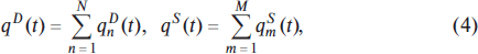
where summing up of quantity quotations is executed formally for the market, which consists of N buyers and M sellers. In this case we understand that for the whole market we can draw all the same pictures as displayed in Figs. 1–6 for the two-agent market. Thus, for instance, we can represent the dynamics of our many-agent market by the help of the following pictures in Fig. 7. In it, the dynamics of many-agent market are depicted at the moment of equilibrium (curves qD(pD) and qS(pS)), as well as dynamics of the stationary economy (point E) and dynamics of the non-stationary growing and falling economies.
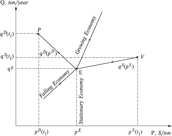
Fig. 7. Dynamics of the many-agent market economy in the price-quantity space. qD(pD) and qS(pS) are quantity trajectories reflecting dynamics of market agents’ quotations in time up to the moment of establishment of the equilibrium and making transactions at the equilibrium price.
4.4. The Classical Economies versus Neoclassical Economies
Let us call attention to the fact that, in Figs. 3 and 6, the quotation curve of the buyer, q1D (pD), has negative slope, and the slope of the quotation curve of the seller, q1S (pS), is positive. This reflects the natural desire of the buyer to purchase more at the lower price, as far as possible, and the natural desire of the seller to sell more at the higher price, as far as possible. Specifically, it is here we reveal the visual similarity of the classical economies to the known neoclassical model of S&D. But the visual similarity of picture in Figs. 3, 6 with the corresponding famous neoclassical picture in the form of two intersected lines of S&D is only formal; economic content in them is entirely different. In classical economies, this is a graphic representation of the real market process (which really occurs on the market at a given instant), while in the neoclassical economies, this picture expresses the planned actions of market agents on the market in the future. Note that in neoclassical economics it is namely the curves qS(pS) and qD(pD) that are called S&D functions. The economic content of these S&D functions can be roughly expressed thus: “the market is by itself, I am by myself”. If one price is on the market, then I purchase (or I sell) one quantity, and if it is another, then will I purchase (or I will sell) another quantity, and so forth. Thus, the market process is completely ignored in the neoclassical economic model. But we know that, in real market life, all market agents participate continuously in the market process, permanently changing price and quantity quotations, since each has made transaction price changes on the market. We will discuss neoclassical models in more detail in other chapters of the book. However, we will now develop an artificial classical economy that will be as similar to the neoclassical model as possible.
We will call this model the quasi-market economy with the “visible hand of the market” in order to distinguish it from the economies having self-organizing markets, or economies that exhibit the “invisible hand of market”. In the quasi-market economy, there is a definite chief (very strict and all-seeing by definition) of the market (visible hand of the market), to whom all agents of the market for the planned period, let us say a year, must pass very detailed and reliable plans with respect to purchase and sale of goods. These plans are compiled by agents and are given to the chief in the form of tables, which are formed according to the rule stated above. If just such a price is found on the market, then I will sell a particular volume; if it is another price, then I will purchase (or sell) another, specific volume, and so forth. These agent tables are represented in Fig. 8 for simplicity in the form of continuous straight lines, a factor which does not decrease their generality in this case.
Let us note that each agent passes its plan to the chief in the form of table, and chief itself unites data of these plans and presents them in the easy-to-use shape of the two straight lines in one picture. Common sense tells us that it is most profitable for the buyer to purchase more at the minimum price. But in this scenario the seller would want to sell less. The opposite would be true for both buyer and seller at the maximum price. Graphically, this is reflected in the fact that when point P1 is higher than point V1, and the point V2 higher than point P2, the consequence is that the slope of the curve of the buyer is be negative, and the slope of the curve of the seller, positive. It is obvious that these two straight lines will compulsorily be crossed at the point E (pE, qE), where the prices and quantities of the buyer and seller coincide. Next, the chief considers that these prices and quantities reflect certain equilibrium in the market, he or she calls the equilibrium price and quantity and declares that these values of price and quantity are set for the market year. Market process is, in this case, further completely eliminated from market life, in that the decisions of the market's chief completely substitutes it during the next year. We call this model economy a quasi-market one, since plans are compiled by market agents. However, they realize them in the prices and the quantities that are essentially dictated by the market’s chief.
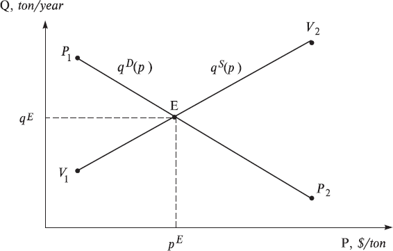
Fig. 8. The classical two-agent quasi-market economy in the economic price-quantity space.
We consider this quasi-market, stationary classical economy to be, in essence, the neoclassical model of S&D. The graphic representation of the neoclassical model economy is, by the way, the same Fig. 8, since plans in the neoclassical theory are drawn up in precisely the same way that we described above for the quasi-market economy. But in neoclassical economics, it is considered a priori that the market itself in some manner will carry out the role, which the chief of the market fills in the quasi-market economy. But if the market process is absent and there are no actions of agents adapting to the market, then who or what will fill this role? Moreover, if the economy is in a stationary state, then all prices and quantities are already known to all participants in the market, and their plans then are graphically reduced simply to one point: E. It is here that the neoclassical model generally lacks any sense or value.
References
1. A.V. Kondratenko. Physical Modeling of Economic Systems. Classical and Quantum Economies. Nauka, Novosibirsk, 2005.
CHAPTER II. The Constructive Design of the Agent-Based Physical Economic Models
“The specific method of economics is the method of imaginary constructions… Everyone who wants to express an opinion about the problems commonly called economic takes recourse to this method… An imaginary construction is a conceptual image of a sequence of events logically evolved from the elements of action employed in its formation. It is a product of deduction, ultimately derived from the fundamental category of action, the act of preferring and setting aside. In designing such an imaginary construction the economist is not concerned with the question of whether or not it depicts the conditions of reality which he wants to analyze. Nor does he bother about the question of whether or not such a system as his imaginary construction posits could be conceived as really existent and in operation. Even imaginary constructions which are inconceivable, self-contradictory, or unrealizable can render useful, even indispensable services in the comprehension of reality, provided the economist knows how to use them properly. The method of imaginary constructions is justified by its success. Praxeology cannot, like the natural sciences, base its teachings upon laboratory experiments and sensory perception of external objects… The main formula for designing of imaginary constructions is to abstract from the operation of some conditions present in actual action. Then we are in a position to grasp the hypothetical consequences of the absence of these conditions and to conceive the effects of their existence… The method of imaginary constructions is indispensable for praxeology; it is the only method of praxeological and economic inquiry”.
Ludwig von Mises. Human Action. A Treatise on Economics. Page 236
PREVIEW. What is the Physical Economic Model?
This is the conceptual mathematical dynamic model of the many-agent economic systems in the formal space of the independent variables, prices and quantities, of all the market agents. It is built through a significant analogy with the theoretical physical models of the many-particle systems in real space, but taking consistently into account basic, specific differences in the economic and physical systems. Each model is, in essence, only an imaginary construction, which by no means completely reflects genuine reality. It is, however, capable of describing one or several basic special features of structure or functioning of the market economy in sufficiently strict mathematical language. It was primarily created to provide fresh insight into these features, and, after the addition of another model feature or interaction, to understand, precisely how it influences entire end results.
1. The Basic Concept of Physical Economic Design
By stretching a point, we can say that the basic concept of design of our physical economic models is skeuomorphism. Let us explain what this concept means in our case. As we have already mentioned repeatedly in this book, when constructing physical economic models we strive to reach a formal mathematical, linguistic and even graphical similarity to their physical prototypes. Specifically, this concerns both the structure and the dynamics, as well as the language and the methods of representation of the obtained results, including graphics. We consistently follow this basic concept of design throughout the book. Let us stress another point. Our main task in the book is the construction of economic models that, in as much as possible, highly resemble or copy the known form and custom physicists’ models of many-particle systems. This facilitates understanding of the models and makes it possible to use the existing, detailed language of physics within a new economic framework. For example, the language of wave functions and probability distributions will be widely used here below, although this, of course, unavoidably leads to the appearance in the theory of a large quantity of neologisms. This may strongly hamper the reading of texts by economists, but substantially facilitates this process for specialists in the fields of natural sciences. We think that this basic design concept is quite adequate for building physics-based models of economic systems.
We begin with the requirement that the graphical scheme of the physical models must be similar to the picture of the many-particle physical systems, such as polyatomic molecules, for instance. Main elements of our physical models of economic systems are shown schematically in Fig. 1. A large sphere covers a market subsystem or economy consisting of active market subjects: buyers who have financial resources and a desire to buy goods or commodities, and sellers who have goods or commodities and a desire to sell them. They are the sellers and the buyers who form supply and demand (S&D below) in the market. Small dots inside the sphere denote buyers, and big ones denote sellers. The cross-hatched area outside the sphere represents the institutional and external environments, or more exactly, internal institutions such as the state, government, society, trade unions etc., and the external environment including other markets and economies, natural factors etc. It is evident that all elements and factors of the system influence each other; buyers compete with each other in the market for goods and sellers compete with each other for the money of buyers. Buyers and sellers interact with each other, permanently influencing each other’s behavior. Institutions and the external environment influence all the economic agents, including not only businesses but also ordinary people. In other words, all the economic agents are influenced by institutional and external environments and interact with each other.
Fig. 1. The physical model scheme of an economic system: a market consisting of the interacting buyers (small dots) and sellers (big dots) who are under the influence of the internal institutions and the external environment beyond the market (covered by the conventional imaginary sphere).
In order to develop a physical model of the economic system, it is necessary to learn to describe in an exact, mathematical way both movements (behaviors and influences) of each economic agent, i.e., buyers and sellers, the state and other institutions etc., and interactions with each other. It is the goal to derive equations of motion for market agents – the buyers and sellers – who determine the dynamics, movement, or evolution of the market system in time.
2. The Economic Multi-Dimensional Price-Quantity Space
As we already discussed above, in order to show the movement or dynamics of an economy it is necessary to introduce a formal economic space in which this movement takes place. As an example of such space we can choose a formal price space designed by the analogy with a common physical space. We choose the prices Pi of the i-th item of goods as coordinate axes: i = 1, 2,…, L, where L is the number of items or goods (the bold P will designate below all the L price coordinates). In case there is only one good, the space is one-dimensional and represented by a single line. The coordinate system for the one-dimensional space is shown in Fig. 2.
The distance between two points in one-dimensional space p' and p" can be for instance determined by the following:

If two goods are traded on the market (L = 2), the space is a plane; the coordinate system is represented in this case by two mutually perpendicular lines (see Fig. 3).
The distance between two points p' and p" can be determined as follows:

We can build the price economic space of any dimension L in the same way. In spite of its apparent simplicity, the introduction of the formal economic price space is of conceptual importance as it allows us to describe behavior of market agents in general mathematical terms. It represents realistic occurrences, as setting out their own price for goods at any moment of time t is the main function or activity of market agents. It is, in fact, the main feature or trajectory of agents’ behavior in the market. Let us stress once again that it is our main goal to learn to describe these trajectories or the distributions of price probability connected with them. It is impossible to do this in a physical space. For example, we can thoroughly describe movement or the trajectory of a seller with goods in physical space, especially if they are in a car or in a spaceship. However, this description will not supply us with any understanding of their attitude towards the given goods; nor will it explain their behavior or value estimation regarding the goods as an economic agent.

Fig. 2. The economic one-dimensional price space for the one-good market economy.

Fig. 3. The economic two-dimensional price space for the two-good market economy.
Within the problem of describing agents’ behavior in the market, the role of the good prices P as independent variables, or a coordinates P is considered here to be in many situations a unique one for market economic systems. In these cases we can study market dynamics in the economic price spaces. But market situations occur fairly often in which we need to explicitly take into account the independent good quantity variables Q (the bold Q will designate below all the L quantity coordinates) and consequently to describe economic dynamics in the economic 2×L-dimensional price-quantity spaces. In these scenarios, we can imagine that the whole economic system is located in the multi-dimensional price-quantity space as it is displayed in Fig. 4. We have already used many aspects of this idea naturally when discussing classical economics. We will address any concerns in the upcoming chapters.
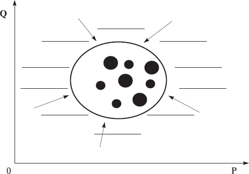
Fig. 4. The graphical model of the many-good, many-agent market economy in the economic multi-dimensional price-quantity space. It is displayed schematically in the conventional rectangular multi-dimensional coordinate system [P, Q] where, as usual, bold P and Q designate the price and quantity coordinate axes for all the goods. Again, our model economy consists of the market and the institutional and external environment. The market consists of buyers (small dots) and sellers (big dots) covered by the conventional sphere. Very many people, institutions, and natural and other factors can represent the external environment (cross – hatched area behind the sphere) of the market which exerts perturbations on market agents (pictured by arrows pointing from environment to the market).
3. The Market-Based Trade Maximization Principle and the Economic Equations of Motion
As we saw above in the example of the simplest classical economies, market agents actively make trade transactions, and there are no trade deals at all out of the equilibrium state. As the inclination of market agents’ action is to make deals, we can naturally conclude that market agents and the market as a whole strive to approach an equilibrium state that can be expressed as the natural tendency of the market to reach the maximum volume of trade. This fact can serve as a guide for using the market agents’ trajectories to describe their dynamics. Moreover, this fact gives us grounds to expect that equations of motion can be derived from the market-based maximization principle, used to describe these trajectories. Specifically, the main market rule “Sell all – Buy at all” can be regarded to some extent as a verbal expression of both the tendency of the market toward the trade volume maximum, and the principal ability to describe market dynamics by means of agent trajectories as solutions to certain equations of motion.
The second reason of we have confidence in creating a successful dynamic or time-dependent theory of economic systems in the economic spaces is based on the analogous dynamic theory of physical systems in physical space. We also admit that the reasonable starting point in the study of economic systems dynamics is with equations of motion for a formal physical prototype. This is in spite of the differences between the features of the economic and physical spaces and the features of the economic and physical systems. The type of equations in the spaces of both systems will be approximately the same, though the essence of the parameters and potentials in them will be completely different. It is normal in physics that one and the same equation describes different systems. For example, the equation of motion of a harmonic oscillator describes the motion of both a simple pendulum and an electromagnetic wave. Formal similarity of the equations does not mean equality of the systems which they describe.
The discipline of physics has accumulated broad experience in calculating the physical systems of different degrees of complexity with different inter-particle interactions and interactions of particles with external environments. It makes sense to try and find a way to use these achievements in finding solutions to economic problems. Should any of these attempts prove to be successful, it would establish the opportunity to do numerical research on the influence that both internal and external factors exert on the behaviours of each market agent, as well as the entire economic system’s activity. This process would be done with the help of computer calculations done on the physical economic models. Theoretical economics will have acquired the most powerful research device, the opportunities of which could only be compared to the result of the discovery and exploration of equations of motion for physical systems.
The next step in developing a physical model after selecting an appropriate economic space, is the selection of a function that will assist us in describing the dynamics of an economy, such as the movement of buyers and sellers in the price space. Trajectories in coordinate physical space x(t) (classical mechanics), wave functions ψ or distributions of probabilities |ψ|2 (quantum mechanics), Green’s functions G and S-matrices (in quantum physics), etc. are used as such functions in physics. We started above with an attempt to develop the model using trajectories in the price space p(t) by analogy with the use of trajectories x(t) of point-like particles used in classical mechanics. Below, this model is referred to as a classical model or simply, a classical economy. Below, we will use the term classical economy in the broad sense for designating the branch of physical modeling of many-agent economic systems with the help of methods of classical mechanics of many-particle systems. It is important to realize that each selection gives rise to its own equations of motion and, therefore, to different physical economic models. For example, if we select from these trajectory variants, then we obtain the economic Lagrange equations of motion and, therefore, the classical economies as the physical economic models. The discussion will deal with these models in detail in Chapter III. If we select wave functions, then we obtain at the output the economic Schrödinger equations of motion and, therefore, quantum economies (see Chapters IX and X). Without going into details here, let us say that both the Lagrange and Schrödinger equations appear as the result of applying the principles of maximization to the whole economic system. This is analogous to the maximization principles, which are explored in physics in obtaining the Lagrange and Schrödinger equations, respectively.
Strictly speaking, all these principles of maximization, both in economics and physics, are in essence a set of hypotheses. Their validity or effectiveness can be confirmed only via practical calculations and comparison of their results with the respective known laws and phenomena, as well as with the relevant big empirical data. But intuition suggests that this way of developing economic theory is most optimum at the present time. Since it is presently not known how to derive equations of motion in economics, borrowing existing theoretical structural models from physics is helpful. Since analogies can be drawn between the spaces and features of both physics and economics, we can use skeuomorphism and transfer the design models from the one discipline to the other.
We understand that in principle, equations of motion for economics can be derived with the aid of the market-based trade maximization principle. To be honest, we do not fully understand how this exactly works. According to some indirect signs, we can only surmise that the market-based trade maximization principle and maximization principles borrowed from physics, work in one direction. We will examine this more specifically in Chapter VIII.